

Where the Curves Cross


One of my all-time favorite papers is from Andrew Ng and Michael Jordan: “On Discriminative vs. Generative Classifiers: A Comparison of Logistic Regression and Naive Bayes.” Advances in Neural Information Processing Systems 14 (2001). It was ten years old when I first read it when I was a postdoc in 2011, and it’s 25 years old now. It’s a beautiful paper, and I keep returning to it because it captures a pattern I see everywhere in machine learning and robotics.
The paper explores Naive Bayes (remember Naive Bayes? The advent of Spam filtering!) and Logistic Regression. These two models are used for discrete classification and make the same conditional independence assumption.
Naive Bayes estimates these probabilities by counting and multiplying. Logistic regression instead directly estimates the conditional distribution. How can we model this conditional distribution? As Tom Mitchell explains in Machine Learning (1997) in section 3.1, the parametric form can be derived directly from the conditional independence assumptions we make for Naive Bayes, as the precise exponential form of the logistic function. We can even use the Naive Bayes assumptions to estimate the logistic feature weights to produce the same result as the Naive Bayes estimator. But we can also estimate the weights directly, for example, by choosing weights that maximize the conditional data likelihood via gradient descent.
Here is the key observation: in this sense, logistic regression searches over a larger space of models than Naive Bayes. Naive Bayes builds in more structure. Logistic regression is more flexible.
The Crossing
Ng and Jordan provide theoretical and empirical results showing that this leads to two distinct performance regimes. When the dataset is small, the more structured model (Naive Bayes) outperforms Logistic Regression because it leverages its assumptions to learn from fewer data points. When the dataset is large, Naive Bayes asymptotes to a higher error rate than Logistic Regression. The curves cross.
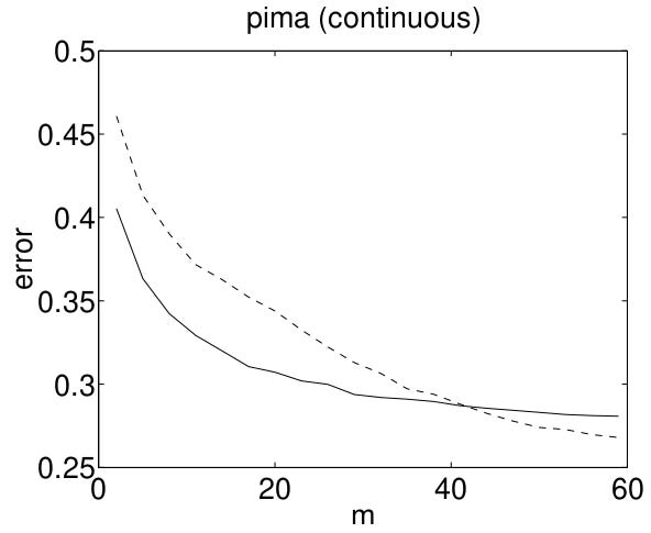
In this figure which is quoted from Ng and Jordan’s paper, the X-axis shows dataset size, and the Y-axis shows classification error (lower is better). The solid line is Naive Bayes, the dotted line is Logistic Regression.
This graph shows that as we add more data to the training set, test set accuracy improves for both methods. In the low-data regime, the more structured model outperforms. As we add more data, the model with less structure fits the distribution better and asymptotes lower. There are two performance regions, one in the low-data regime, and one in the high-data regime.
This is the insight that changed how I think about model selection: it isn’t that Naive Bayes is better and Logistic Regression is worse. Both methods are more effective in certain zones. The question is which zone you’re operating in.
Why This Matters for Robotics
I’ve found this pattern to be constantly relevant in robotics. Models with more structure can outperform with less data (consider the work by Rob Platt and his collaborators on equivariance), especially when the structure is somewhat correct. Models with less structure need much more data but can asymptote to higher values (i.e., the bitter lesson).
In my lab reading group, we recently read “Inquire: Interactive Querying for User-Aware Informative Reasoning” by Tesca Fitzgerald et al. The paper addresses a practical question: what kind of input should an algorithm request from a person to train a skill? The options include demonstrations (showing the robot what to do), preferences (choosing between two trajectories), corrections (modifying a trajectory), or binary questions (is this trajectory okay?).
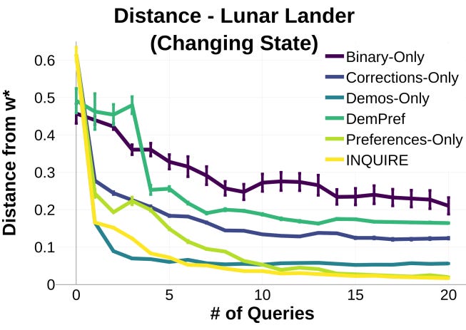
In this graph quoted from Tesca’s paper, the X-axis is the number of queries, Y-axis is the distance from the optimal policy (lower is better)—multiple lines for different query types.
We see the same crossing phenomenon. The Demos-only line corresponds to using only behavior cloning. It asymptotes quickly but does not achieve optimal performance. The Preferences-Only line corresponds to asking a person to choose which of two trajectories they prefer, more like on-policy RL with a dense reward function. This method asymptotes more slowly, so with fewer queries, the behavior cloning approach is better. But for more than 10 queries, the preference-based approach outperforms behavior cloning because it is free to search outside the demonstrations for an optimal policy.
The method described in the paper, INQUIRE, gets the best of both worlds: it relies on demonstrations to perform well with less data, then uses preferences to achieve lower asymptotic error. With only 20 demonstrations in total, we are far from the “large data regime” on this task, making the hybrid approach particularly valuable.
A Framework for Thinking About Model Selection
Observing where curves cross changes helps us change from black-and-white thinking to recognizing there is a spectrum of approaches with trade-offs at each end. This perspective opens research questions beyond “more data.” The questions become: Does your task have a well-defined structure that you can encode in a model? Do you have lots of data and compute? And perhaps most interesting: how can we find the right structure for robotics problems that enables data- and compute-efficient learning without sacrificing asymptotic performance?
Thanks to Jessica Hodgkins for comments on earlier drafts of this post. Any errors that remain are our own.