

What Babies Know That Robots Don’t
On tokenization, biological Fourier transforms, and becoming data engineers


I watched Episode 4 of Netflix’s Babies documentary, expecting cute footage, and ended up thinking about representation learning for three days.
The episode follows researchers studying how infants crack language. Babies sit in labs, headphones on, listening to streams of made-up syllables. “Pabiku, golatu, tibudo, daropi, pabiku…” No pauses. No visual cues. Just sound. And after two minutes, these eight-month-olds can tell which three-syllable chunks belong together.
They’re tokenizing raw audio before they can speak words.
The Saffran Experiment
In 1996, Jenny Saffran and colleagues at the University of Rochester (where Stefie grew up!) ran a now-famous experiment. They created four nonsense “words.” Pabiku, tibudo, golatu, and daropi. They concatenated them into a continuous stream. Within each word, the transitional probability between syllables was 1.0: pa always leads to bi, bi always leads to ku. Across word boundaries, the probability dropped to 0.33: ku could be followed by ti, go, or da.
After just two minutes of exposure (about 45 repetitions of each word), infants could distinguish the “words” from “part-words” like tudaro (spanning the boundary between golatu and daropi). The only information available was the statistical structure of syllable co-occurrence.
The researchers describe this as babies finding correlations in sounds. I immediately thought of tokenization and attention. It is the same statistical structure that transformers exploit, discovered twenty years earlier in infant cognition.
What’s Actually Happening
By the time a baby sits in Saffran’s lab, that child has already spent months building powerful abstractions about sound. The cochlea has been decomposing pressure waves into frequency bands. The auditory cortex has been learning what similar sounds mean. The two minutes of nonsense syllables aren’t learning from scratch, but instead applying the already-developed representations to a new domain.
Patricia Kuhl, a researcher at the University of Washington, showed that babies are taking statistics on the sounds around them from the moment they can hear. This includes time spent in the womb. Newborns show a preference for their native language within days of birth (Moon et al. 1993), and by six months, infants in Seattle and Stockholm already perceive vowels differently, tuned to the distributions in their respective languages. The infrastructure for statistical word learning is built before word learning happens.
This is closer to test-time fine-tuning than to training from scratch, or maybe to in-context learning, if you prefer the LLM framing. The baby arrives at the experiment with a foundation model of auditory processing, and the two minutes of pabiku golatu are just a prompt.
The Inner Ear is a Fourier Transform
One detail from the documentary stuck with me: the researchers mention that babies are hearing the ongoing melodies of speech as a flow of the environment. Before understanding any words, they’re sensitive to prosody, the pitch contours and rhythms that segment speech into phrases.
This detail points to something important. The cochlea, that snail-shaped organ in the inner ear, is a biological Fourier transform. Different positions along its length resonate to different frequencies. When sound enters, it’s physically decomposed into frequency bands by the structure of the organ itself. Babies don’t hear raw air pressure fluctuations, but instead something akin to how an engineer uses a spectrogram to analyze the fluctuations in sound over time.
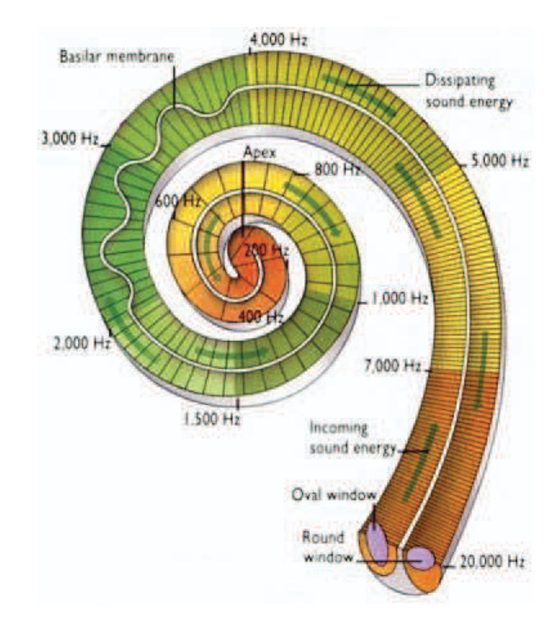
[FIGURE: Diagram of cochlear tonotopy—the base responds to high frequencies, the apex to low frequencies] Figure from Smimite, A. (2014). Immersive 3D sound optimization, transport, and quality assessment (Doctoral thesis). Université Sorbonne Paris Nord, France.
The cochlea’s frequency decomposition is a bias built into our collective wetware, a structure adapted from evolutionary processes rather than something trained.
An Experiment
I wanted to see if this matters, so I ran a simple experiment replicating the Saffran structure. I generated synthetic syllables as combinations of two frequencies, concatenated them into “words” and “part-words” following the same transitional probabilities, and trained simple classifiers to distinguish them. The main factor I wanted to test was how the effectiveness of the learning changed when I transformed the audio signal differently.
Here are the five different, non-exhaustive ways we could process audio information:
Raw Waveform: The audio signal as-is—amplitude over time. A 450ms word at 16kHz is 7,200 numbers representing air pressure fluctuations. The problem: phase shifts destroy structure. The same syllable starting at a different point in time looks completely different, even though it sounds identical.
Spectrogram (STFT): Short-Time Fourier Transform. We slide a window across the signal and compute the frequency content at each position. This gives us a 2D image: time on one axis, frequency on the other, intensity as brightness. Now, the phase doesn’t matter as we see what frequencies are present at each moment.
Mel Spectrogram: Same as spectrogram, but frequencies are warped to match human perception. We hear the difference between 100Hz and 200Hz more easily than between 8000Hz and 8100Hz. The mel scale compresses high frequencies, mimicking the cochlea’s logarithmic frequency response.
MFCC (Mel-Frequency Cepstral Coefficients): Take the mel spectrogram, apply a log transform, then take the DCT of each frame. This captures the “shape” of the spectrum, roughly corresponding to vocal tract configuration, while discarding fine spectral detail. This has been standard in speech recognition for decades.
DCT of Waveform: Apply the Discrete Cosine Transform directly to the raw waveform. This decomposes the signal into frequency components, but globally across the entire duration. Unlike the spectrogram, there’s no time localization. A syllable at the start vs. the end of the word produces very different coefficients. It’s the wrong tool for a sequential structure. We show this because it is important to see that hiding these components doesn’t provide enough information to the neural network to allow it to learn.
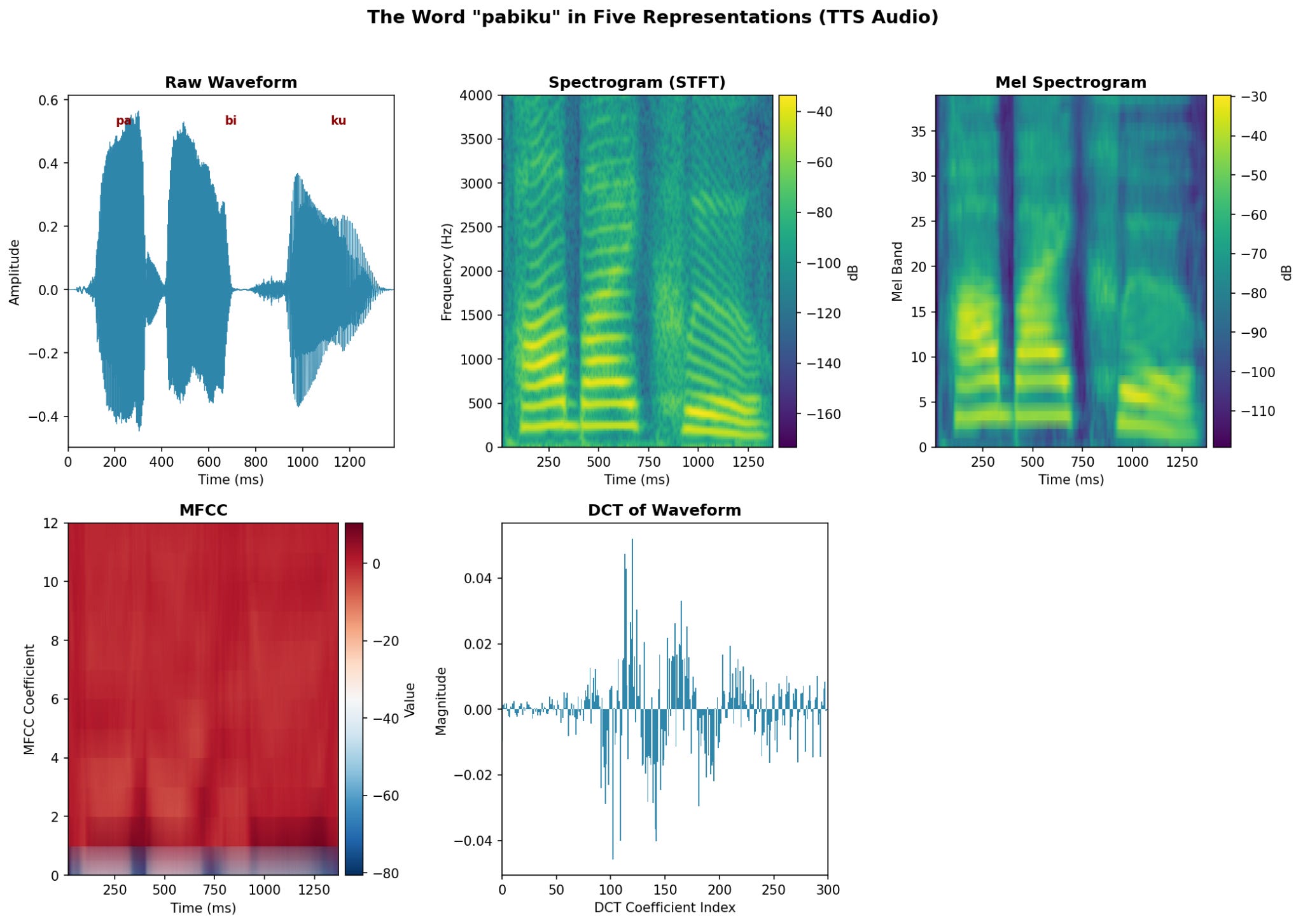
[FIGURE: Side-by-side visualization of “pabiku” in all five representations]
Results: Synthetic Tones
Here are the results of our synthetic tones

Using the raw waveform doesn’t even beat chance. The classifier is trying to find statistical structure in a representation that doesn’t make that structure visible. The mel spectrogram with frequencies weighted the way the cochlea weighs them trivializes the task.
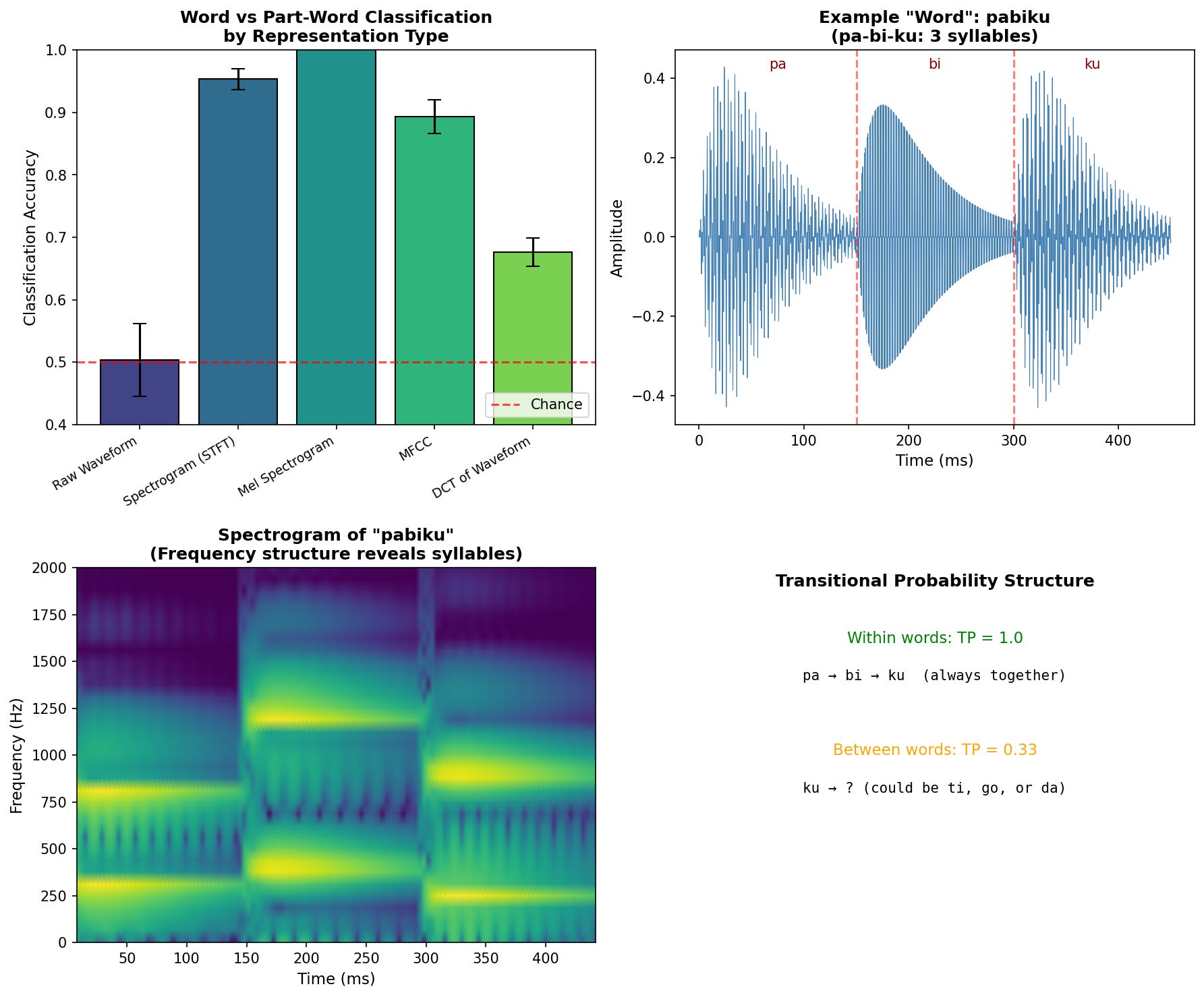
The DCT destroys the exact information we need. The Saffran task is about the sequential structure of which syllable follows which. But the DCT treats the entire word as a single unit and asks, “What frequencies are present overall?” without preserving temporal order. It’s the wrong decomposition for a task that depends on sequence. At least the raw waveform preserves time, even if it encodes it poorly.
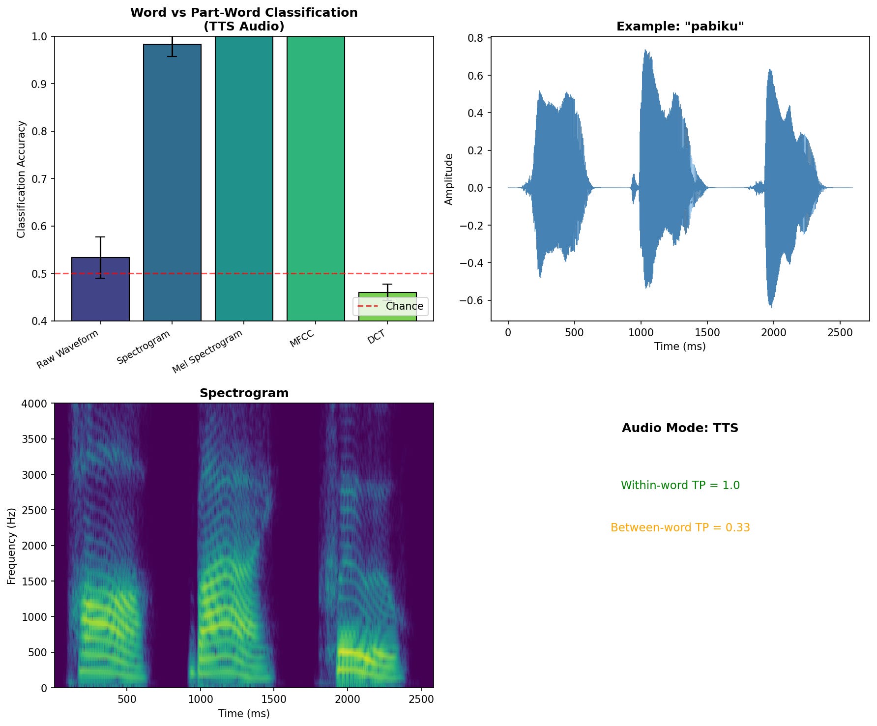
Verification with Text-to-Speech
To confirm these results weren’t an artifact of my synthetic tone generation, I ran the same experiment using Google’s text-to-speech engine to produce actual spoken syllables.
Example word "pabiku" - synthetic tones
Example word “pabiku” - TTS
Example part-word “tudaro” - synthetic tones
Example part-word “tudaro” - TTS
Training stream sample (10 words concatenated)
The pattern holds with synthetically generated speech:
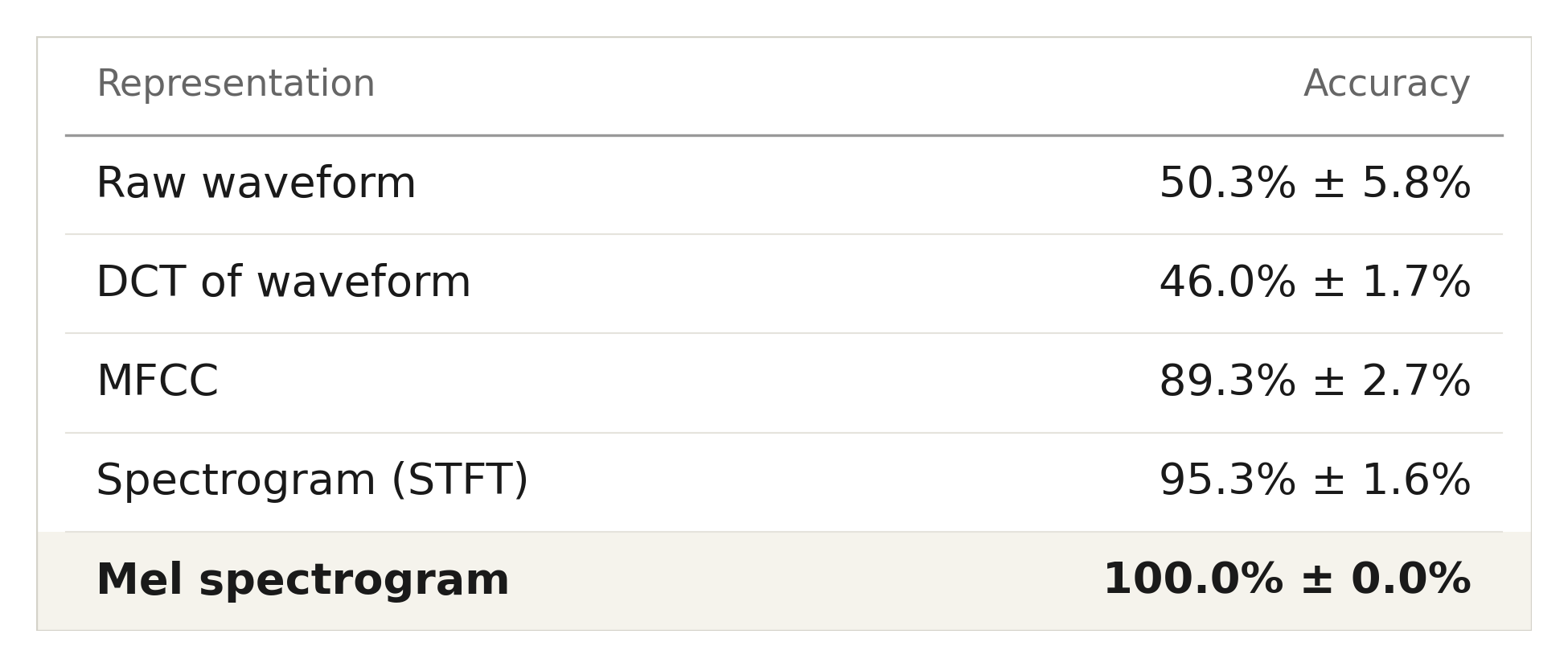
Interestingly, MFCCs perform slightly worse with real speech than with synthetic tones. This makes sense because MFCCs were designed to capture phonetic identity while being invariant to speaker characteristics. That invariance throws away some of the information that distinguishes our artificial words. The mel spectrogram, which preserves more raw spectral detail, handles both cases perfectly.
The Implication for Robotics
The cochlea is evolution’s answer to the audio representation problem. We spend considerable effort in robotics designing clever representations: RGB feature extraction for SLAM, Disparity maps for depth, and grid environments for A* search. These encodings make specific algorithms tractable, but they carry structural biases that may not transfer to learning.
End-to-end learning advocates are having the network discover its own representations. There is some credibility to this, as sensor designers have done significant work making these sensors reliable. For example, the sensors on a camera are tuned for what a human eye is going to perceive, and our eyes are good enough to solve tasks we do every day. But it is not obvious that this is going to transfer to things we don’t do well, such as handling extremely hot materials. Similarly, it is not obvious that we should pass a spectrogram into a CNN for audio processing; indeed, wav2vec 2.0 and similar models bypass the spectrogram entirely, learning directly from raw waveforms.” The translational invariance that makes CNNs powerful for images doesn’t work when your axes (time and frequency) have fundamentally different semantics. The representation should match the structure of the problem.
Infants have an advantage over our synthetic sensors: evolution produced a cochlear design that makes statistical learning over acoustic sequences efficient. The representation is not neutral and is designed to make specific statistical structures, such as the sound of a mother’s voice, discoverable. If we want robots to learn as efficiently as infants, we need to think harder about whether our sensor outputs are the right substrate for learning.
Diversity Over Volume
Here’s a thought experiment. A thousand hours of warehouse piece-picking, or a thousand one-hour experiences across radically different contexts? Which is going to result in better performance for that warehouse piece-picking task?
Obviously, the warehouse-only data will win if you evaluate narrowly on the warehouse distribution it was trained on. The interesting test is what happens when the boxes are slightly different, the lighting changes, or a novel object appears. That’s where the diverse-experience system should pull ahead, because it has been forced to learn what’s invariant. The paper tears like fabric. The sand flows like rice. These cross-domain regularities are precisely what make cognition transferable.
We should be collecting data that forces this kind of abstraction. We should collect diverse experiences that require the model to discover what’s invariant across contexts.
Curriculum and Abstraction
Kathy Hirsh-Pasek’s research, featured in the documentary, shows that passive exposure to language is not enough. Children who engage in back-and-forth interaction show stronger language development than those who simply hear language spoken around them. Children actively test hypotheses and need feedback to refine them.
Infant-directed speech illustrates this scaffolding: the elongated vowels and exaggerated pitch contours make statistical structure more salient, helping infants discover word boundaries and phonetic categories.
The same logic applies to how experience is sequenced. Current policies are largely memoryless, but many tasks require temporal context and, more importantly, scaffolds gradually build complexity. The documentary shows bilingual infants separating languages based solely on characteristic patterns, but this works because they’ve already built an infrastructure for discovering statistical structure. We should present robots with increasingly difficult concepts within their current representational capacity. Vygotsky called this the zone of proximal development, and the same principle applies to machine learning: present the system with concepts just beyond its current representational capacity.
The Real Work
The babies in the documentary are doing something remarkable, but they’re not magic (well, actually, they are magical, but the computations the speech-processing parts of their brains are doing aren’t magical). They arrive with hardware optimized for certain kinds of statistical learning. They receive input scaffolded by caregivers who unconsciously adjust their speech to be learnable. They actively explore their environment rather than passively receiving demonstrations.
We don’t have millions of years of evolution to design our sensor suites. But we can carefully consider the representations we’re providing, how we’re sequencing experience, and whether our data-collection methods actually capture the information needed to learn the abstractions we want.
The documentary left me with a simple conclusion: we should all become data engineers. We need to understand that the representation is part of the problem. The curriculum is part of the problem. The diversity of experience is part of the problem.
We must do the hard work of producing data, not just the cool work of consuming it.
References
Saffran, J.R., Aslin, R.N., & Newport, E.L. (1996). Statistical learning by 8-month-old infants. Science, 274(5294), 1926-1928.
Kuhl, P.K. (2004). Early language acquisition: cracking the speech code. Nature Reviews Neuroscience, 5(11), 831-843.
Aslin, R.N., Saffran, J.R., & Newport, E.L. (1998). Computation of conditional probability statistics by 8-month-old infants. Psychological Science, 9(4), 321-324.
Warstadt, A., et al. (2023). Findings of the BabyLM Challenge: Sample-efficient pretraining on developmentally plausible corpora. Proceedings of the BabyLM Challenge at CoNLL.
Hirsh-Pasek, K., & Golinkoff, R.M. (1996). The Origins of Grammar: Evidence from Early Language Comprehension. MIT Press.
Fernald, A. (1989). Intonation and communicative intent in mothers’ speech to infants: Is the melody the message? Child Development, 60(6), 1497-1510.
Smimite, A. (2014). Immersive 3D sound optimization, transport and quality assessment (Doctoral thesis). Université Sorbonne Paris Nord, France.
Moon, C., Cooper, R.P., & Fifer, W.P. (1993). Two-day-olds prefer their native language. Infant Behavior and Development, 16(4), 495-500.
Appendix
Representation Experiment with Like Words
https://drive.google.com/file/d/1S_YvsgEDBASTBIir1symxnlbvTNxH1X_/view?usp=drive_link
Representation Experiment with Like Words (TTS)
https://drive.google.com/file/d/1gHHaimWV6Qi5Zlh2u-lDpCCeeHTvNiGo/view?usp=drive_link