


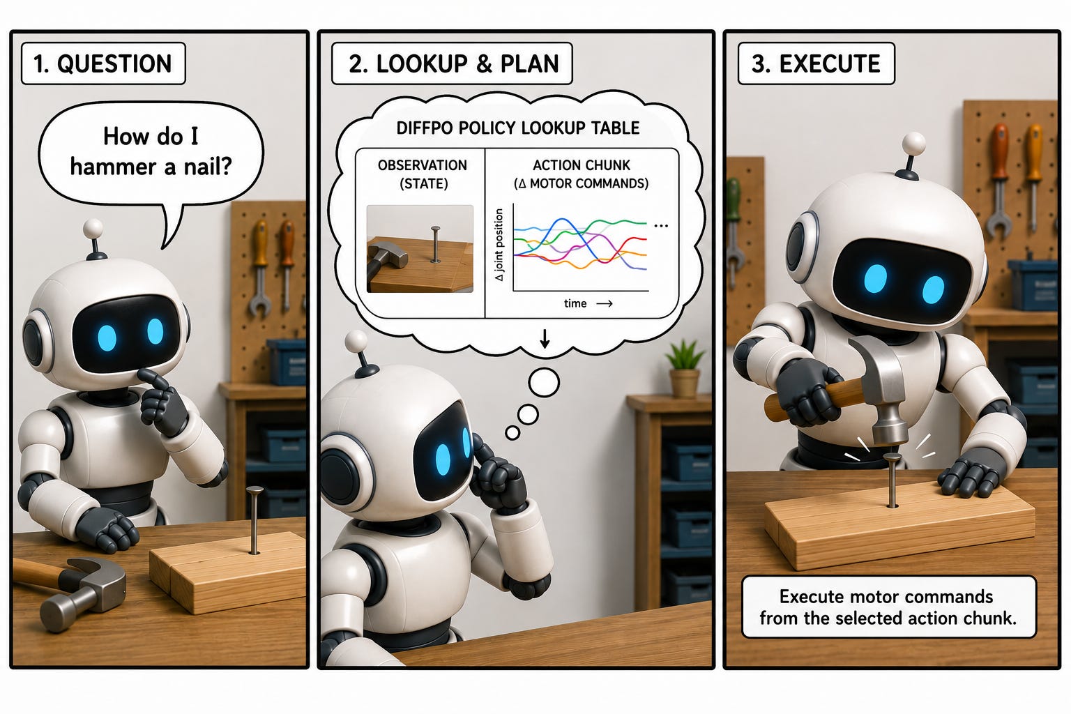
How do you know what data to collect so your robot learns the policy you want? Most answers hide inside talk about what the model "knows" or "understands," language we borrowed from describing people. Ben Burchfield once said a diffusion policy has the memory of a goldfish, since it stays Markov in the state it sees right now. Give up the mentalistic vocabulary and a diffusion policy has a plain mechanical description, and that description tells you what data to go collect. We are still in a pre-paradigm field in robotics, and giving ourselves better vocabulary to describe the phenomena we see helps us do better research. Borrowing language from lookup tables or databases could be a step on that path.
A diffusion policy behaves like a lookup table with good taste. Perception compresses an observation into a latent which serves as a key. The action head takes the key and returns a trajectory drawn from whatever the training data associated with nearby keys. If your lookup table covers the space of keys you expect to see at deployment, then you have trained one of these well. Framing policies this way becomes a strong diagnostic tool. Once you see the policy as a key-and-retrieval system, its failures sort into a small set of named cases to inform what data to collect next.
The Mechanism
A visual encoder extracts the salient content of an image and lands it somewhere in the latent space. Two observations that share task-relevant structure land close together. This creates a mapping that behaves similarly to a hash over the image. The action head holds the trajectories, indexed by where their conditioning landed in that same space. At inference, a fresh observation produces a key, and the head returns the trajectory the neighborhood of that key supports.
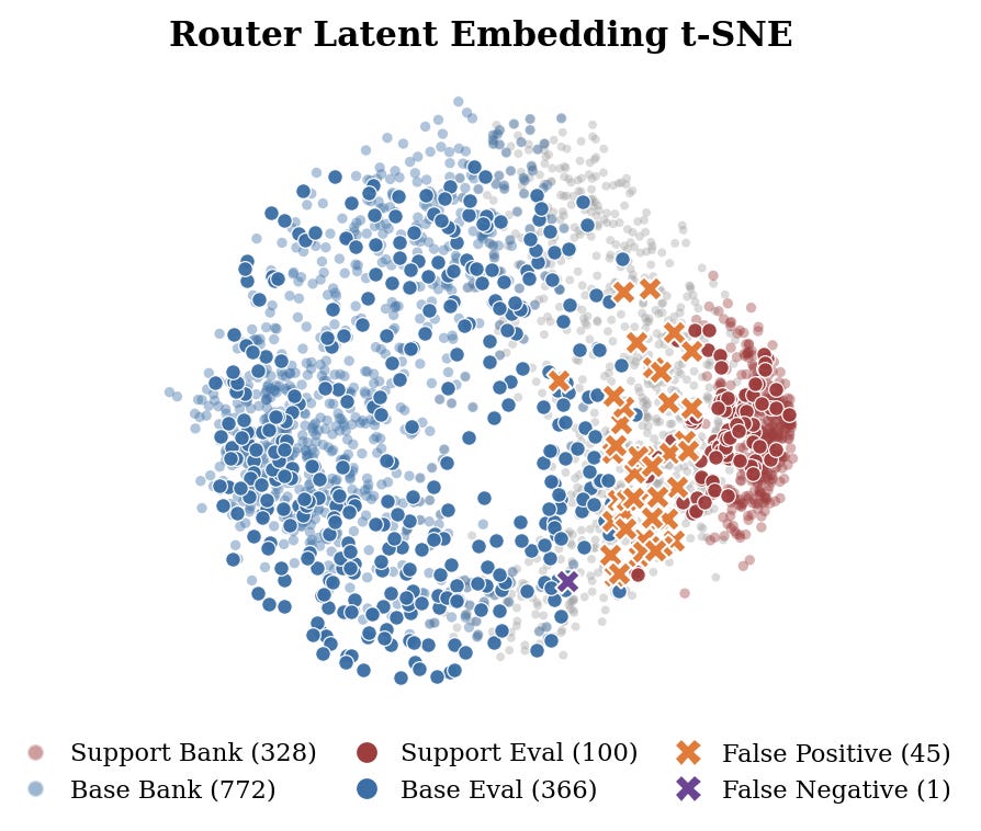
Under this framing, training quality reduces to coverage. A policy works across the region of key space your data fills. Its behavior grows uncertain as you leave that region. You can look at the coverage directly. t-distributed stochastic neighbor embedding (t-SNE) flattens high-dimensional vectors into a 2D picture while keeping neighbors close, which turns the structure of the key space into something you can look at. While t-SNE often doesn't tell you a lot, projecting these latents with t-SNE creates a visual representation of this table: dense clusters where data concentrates, and sparse zones where it thins out. We can see this readily when looking at the distribution of states for known, popular robotics datasets (we should consider making an image to show this).
Coverage is Generalization in Memory Space
A database with full coverage over the input states you care about is generalizing in memory space. We can leverage the existing vernacular to describe databases and their behavior. You can describe a manipulation policy as a series of JOIN operations on different kinds of datasets. We can ask what the coverage costs in big-O, whether we have O(n) space complexity to represent a problem.
A policy can spend memory, covering the key space densely enough that every deployment state finds a close neighbor. It can also spend compute, compressing the space enough that a smaller set of stored structures reproduces the same behavior over a wider region. Diffusion policies as we train them today sit towards the memory end of that axis.This relationship connects to an older idea: learning is compression.
Marcus Hutter pushes that idea to its limit and treats compression and general intelligence as one measurement. An agent that predicts its world well holds a short program that reproduces the data it has seen, and the length of that program indexes how much the agent understands. The Hutter Prize makes this concrete, paying out for smaller lossless encodings of a fixed slice of Wikipedia on the premise that a better compressor carries a better model of the text. Read a diffusion policy through that lens and coverage becomes the surface of a compression problem: the tighter the program that maps keys to trajectories, the more of the deployment space it covers per unit of stored structure.
A policy that stores and retrieves is compressing its training distribution. If we shrink the space we are compressing to too much, we risk dealing with an underparameterized network which starts to behave like a jagged manifold, making learning hard and therefore compressing challenging.
A Diagnostic Framework
There are two stages where mapping from observation to actions can break down.
Collisions: Two states that call for different behavior land on the same key. The head has one entry to return for that key, so it returns one trajectory for both of those states, even though each state needed a different action. We see this behavior in behavior cloning systems as multi-modal behavior or sometimes as averaging depending on the method for example when a robot can pass an obstacle on the left or the right, both routes sit in the data, and a head that regresses the mean averages them into a straight line that drives into the obstacle. Diffusion policies do a better job of picking one of those modes. We can also look at the Markovian nature of the data, and because a single input state maps onto multiple output states, there is a hidden nature to the behavior and therefore the policy is non-Markovian. The encoder discards the information that would have separated those states, or worse yet the researcher that composed the problem and set up the perception stack created an undistinguishable set of states. The fix is a more discriminative key or data that forces the encoder to keep the separating features.
Coverage Gaps: A key lands in a region the table never filled. Retrieval has nothing to return, and behavior there is undefined and erroneous. The fix is to introduce new data that is collected in that region so that the deployment distribution reaches that area. Finding these regions introduces another challenge which is how do we back out what is semantically described by that area? We can use decoders to turn these back into human interpretable regions again.
A coverage gap has an online fix too. If the policy can estimate its own uncertainty, that estimate flags the cells the table never filled. Dodeja and colleagues (including Stefanie!) use this signal directly: their residual RL method reads the base policy's uncertainty and concentrates exploration on the low-confidence regions, learning corrective actions that patch the gap without recollecting a full dataset. The policy notices the empty key and fills the neighborhood around it.Collisions send you toward a better representation. Gaps send you toward more data in a specific place. Both can be viewed from a projection of your data.
What This Looks Like on a Robot
I saw the collision case in the wild through memorization. When I condition the policy on state, such as with cup in the wild in the original UMI paper, the policy will over-attend to velocity and position rather than the image. The head then returned the trajectory the bucket had memorized. Grad-CAM paints a heatmap over the input image showing which pixels moved the policy's output the most, so you can see where it was looking. Utilizing gradCAM can help with determining what salient features your model is biased to looking at over others, but sometimes you just have to look at the policy being deployed on your own hardware.
Where This Leaves Us
Treat the policy as a key-and-retrieval system. You get complexity language for a problem that usually resists it. You get coverage for a picture you can inspect. When behavior breaks, you get a two-way fork, collisions or gaps, that points straight at your next round of data collection. The lookup-table label is a compression over the state of robot behavior that helps us as roboticists do better search.
This is a great article on cutting through the complexity of what (the action head of) a VLA is doing. I love this lens of looking at it - it really demystifies the inherent data issues. I've also been really interested in the lookup table computational classification and how that relates to different types of action heads (e.g. https://www.avikde.me/p/the-loops-and-hierarchies-of-embodied). I'm working on a post on how to view a broader LLM / foundation model from a computational class perspective, as well as a compression lens -- I'll make sure to send people here first!